The Foundation of Large Language Models: Understanding Embeddings in 5 Minutes
I recently revisited Chapter 5 of the NLP “bible”—Jurafsky & Martin’s Speech and Language Processing. This chapter focuses on Static Embeddings, such as Word2vec and GloVe.
You might ask: Doesn’t everyone use BERT and GPT now? Why bother learning “old stuff”?
Because static models are the foundation. Without a solid foundation, you can’t understand the skyscraper built on top.
1. Core Intuition: The Distributional Hypothesis
“You shall know a word by the company it keeps.”
Here’s an example from the book: If an unfamiliar word Ongchoi frequently appears near “garlic,” “delicious,” and “sautéed,” the AI can infer it’s a vegetable (water spinach)—without ever consulting a dictionary.
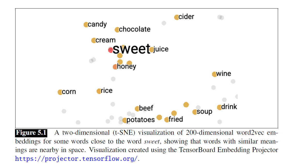 Figure 5.1: In this vector space, words with similar meanings automatically cluster together. Notice how “sweet” is surrounded by “honey”, “candy”, and “chocolate”.
2. Static vs Dynamic: The One-Line Distinction
Static (Word2vec): One word, one vector. The word “apple” always has the same vector, whether it refers to the fruit or the company.
Dynamic (BERT): One word, multiple vectors. The “apple” in “apple pie” and “Apple stock” generates different vectors based on context.
Although static models can’t handle polysemy, they’re fast, cheap, and interpretable—many RAG systems and recommendation engines still use them today.
3. Why Do We Need Embeddings?
Early sparse vectors had dimensions equal to vocabulary size (tens of thousands), with most values being zero.
The biggest problem was “orthogonality”: car and automobile appeared completely unrelated to the model because they occupied different dimensions.
Embeddings (dense vectors) solved this:
- Dimensions compressed to 50-1000
- Semantically similar words are closer in vector space
4. How Do We Measure “Closeness”? Cosine Similarity
Why not use Euclidean distance? Because high-frequency words naturally have longer vectors (more co-occurrences), which would dominate the distance calculation.
Cosine Similarity = normalized dot product. It eliminates the influence of vector length (word frequency), letting us focus purely on semantic direction.
The core formula:
cosine(v, w) = (v · w) / (|v| × |w|)
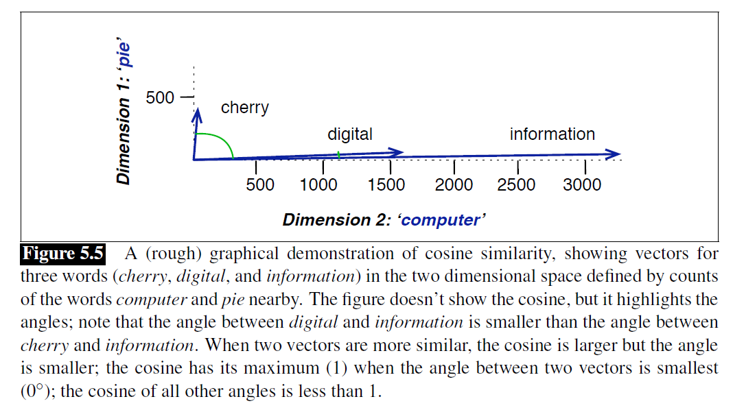 Figure 5.5: The angle between “Digital” and “Information” is small, indicating semantic similarity; “Cherry” points in a completely different direction.
5. The Art of Training Word2vec
Skip-gram is essentially a “pretend game”: it pretends to predict whether a word will appear near another word.
- Self-supervised: No manual labeling needed—the text itself is the answer
- Negative Sampling: A “tug-of-war” process—pulling real neighbors closer while pushing random noise words away
What we want isn’t the prediction result, but the trained weights—that’s the Embeddings.
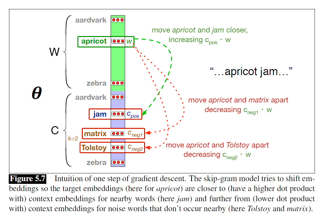 Figure 5.7: The skip-gram model pulls “apricot” and “jam” closer while pushing noise words like “Tolstoy” and “matrix” away.
Pro tip: Word2vec can’t handle words it hasn’t seen during training (the OOV problem). FastText solves this by breaking words into n-gram subwords—even new words can be represented by combining subword vectors.
6. The Other Side of the Coin: AI Bias
Embeddings don’t just learn language—they also learn human stereotypes:
- Classic analogy: King - Man + Woman ≈ Queen
- But the data also taught: Programmer - Man + Woman ≈ Homemaker
Worse still, bias gets amplified in the model. This is the “Allocational Harm” that AI deployment must guard against.
 Figure 5.9: The parallelogram model showing analogy relationships.
Who Needs This Knowledge Most?
- RAG Developers: Cosine Similarity is the core of vector retrieval
- Recommendation System Engineers: Everything can be embedded—compute the distance between users and products
- AI PMs / Compliance: Understand how model bias creates harm, and mitigate ethical risks
- NLP Learners: Understanding Word2vec is the prerequisite for understanding BERT and GPT
From Word2vec to BERT, the underlying logic remains consistent: represent semantics with vectors, measure similarity with distance.
Build a solid foundation, then construct the skyscraper.
Source: Jurafsky & Martin, Speech and Language Processing, Chapter 5